Chapter 10 Venn, Euler, and upSet diagrams
In this chapter, we take a look at R packages and functions to plot sets and their overlaps in R. We will look at 3 visualizations: Venn diagrams, Euler diagrams, and UpSet plots.
10.1 Setup and data
Venn diagrams show all logical relationships between multiple sets.
There is no dedicated function to plot them in base R. Here, we will use
the eulerr package. The demo data comes from the UpSetR package that
we will use more later.
The demo data is a database of movies with genre tags. In this case,
every row contains one movie, every genre is represented by a column.
The fields are filled by 0 or 1. 1 indicates that the movie
belongs to that genre, 0 means that the movie does not belong to the
genre.
movies <- read.csv( system.file("extdata", "movies.csv", package = "UpSetR"), header=TRUE, sep=";" )
head(movies)
## Name ReleaseDate Action Adventure Children
## 1 Toy Story (1995) 1995 0 0 1
## 2 Jumanji (1995) 1995 0 1 1
## 3 Grumpier Old Men (1995) 1995 0 0 0
## 4 Waiting to Exhale (1995) 1995 0 0 0
## 5 Father of the Bride Part II (1995) 1995 0 0 0
## 6 Heat (1995) 1995 1 0 0
## Comedy Crime Documentary Drama Fantasy Noir Horror Musical Mystery Romance
## 1 1 0 0 0 0 0 0 0 0 0
## 2 0 0 0 0 1 0 0 0 0 0
## 3 1 0 0 0 0 0 0 0 0 1
## 4 1 0 0 1 0 0 0 0 0 0
## 5 1 0 0 0 0 0 0 0 0 0
## 6 0 1 0 0 0 0 0 0 0 0
## SciFi Thriller War Western AvgRating Watches
## 1 0 0 0 0 4.15 2077
## 2 0 0 0 0 3.20 701
## 3 0 0 0 0 3.02 478
## 4 0 0 0 0 2.73 170
## 5 0 0 0 0 3.01 296
## 6 0 1 0 0 3.88 940Let’s focus on the 2, 3, and 4 genres with the most movies. We remove movies that don’t belong to those genres (although it’s not strictly speaking necessary).
movies2 <- movies[,c(9,6)] #keep only Comedy and Drama
rownames(movies2) <- movies[,1]
movies2 <- movies2[rowSums(movies2)>0,] #remove movies that are neither Comedy nor Drama

movies3 <- movies[,c(9,6,3)] #keep only Comedy, Drama, and Action
rownames(movies3) <- movies[,1]
movies3 <- movies3[rowSums(movies3)>0,] #remove movies that are neither Comedy nor Drama nor Action

movies4 <- movies[,c(9,6,3,17)] #keep only Comedy, Drama, Action, and Thriller
rownames(movies4) <- movies[,1]
movies4 <- movies4[rowSums(movies4)>0,] #remove movies that are neither Comedy nor Drama nor Action nor Thriller
10.2 Venn diagrams
Plotting is very simple from this format and the default plot looks okay.
plot(venn(movies2))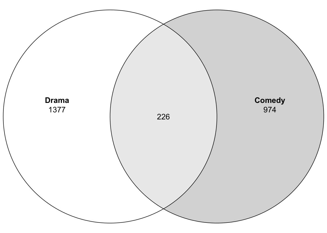
You can adjust the plot, e.g. the colours of the lines and fills:
plot(venn(movies2),edges=c("red","blue"),fills=c("red","blue"))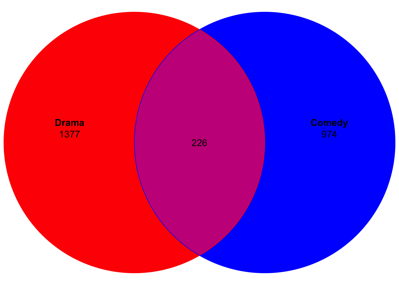
Or just the fills:
plot(venn(movies2),fills=c("yellow","lightgreen"))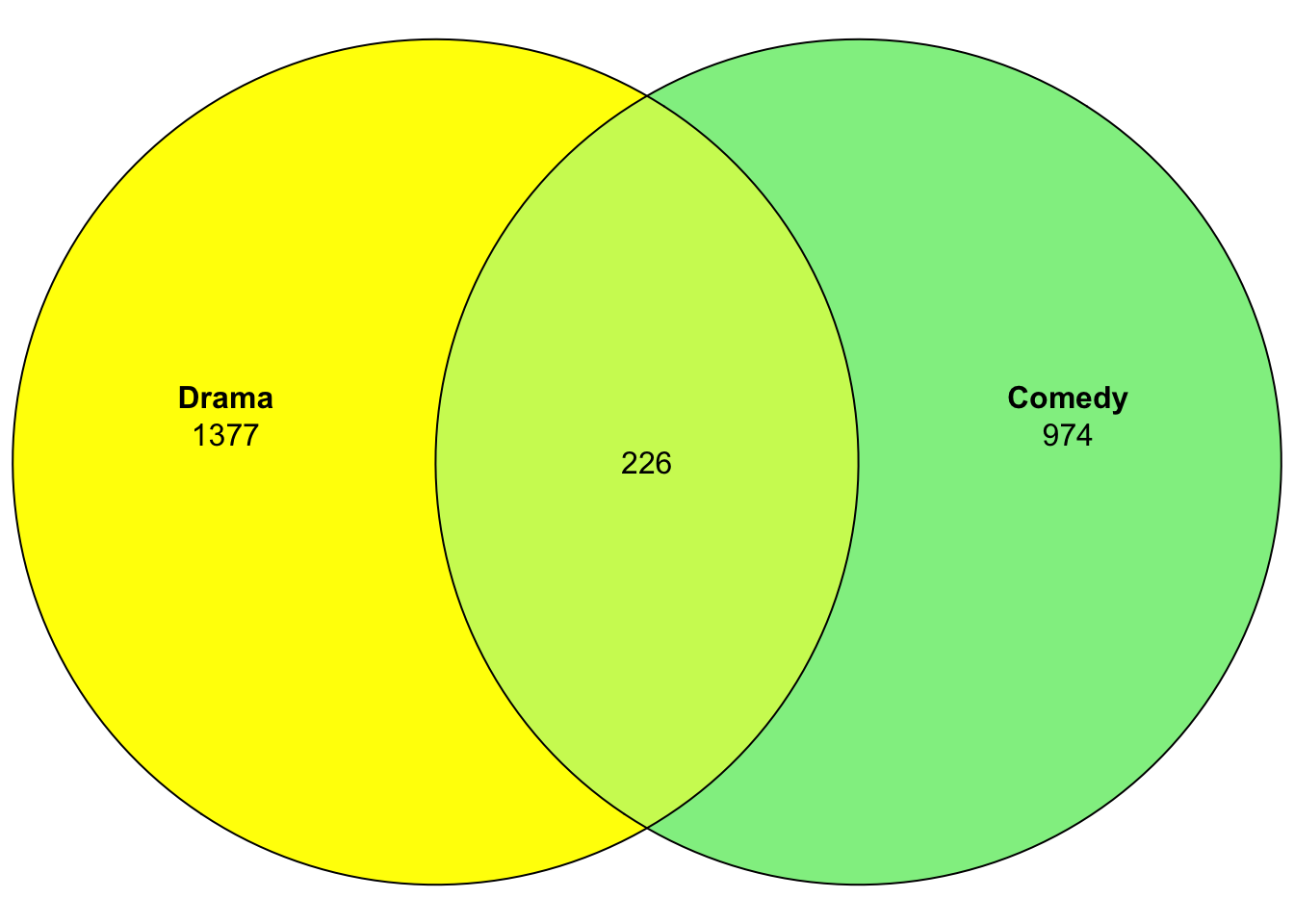
Or the labels:
plot(venn(movies2),fills=c("yellow","lightgreen"),edges=NA,
     labels = c("dramatic movies","comedic movies"))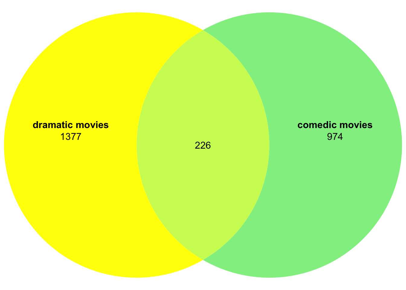
Exercise: try the same in new chunks with the sets of 3 or 4 genres.
Above, we’ve used one kind of input format. The venn function
understands some more formats. You can use them depending on the
original shape of your data. For two groups, this notation can be handy
if you know the intersect sizes already:
movies2_combi_manual <- setNames(c(1377, 974, 226), #values from above
                                 c("Drama", "Comedy", "Drama&Comedy")) #names and intersect with &
plot(venn(movies2_combi_manual),fills=c("yellow","lightgreen"),edges=NA)
Here’s one way to get the numbers automatically:
movies2_combi_A <- sum(movies2$Drama) - length(which(rowSums(movies2)==2))
movies2_combi_B <- sum(movies2$Comedy) - length(which(rowSums(movies2)==2))
movies2_combi_AB <- length(which(rowSums(movies2)==2))
movies2_combies <- setNames(c(movies2_combi_A, movies2_combi_B, movies2_combi_AB),
                                 c("Drama", "Comedy", "Drama&Comedy"))

plot(venn(movies2_combies),fills=c("yellow","lightgreen"),edges=NA)
Or, if your sets are not available as a table, but rather as a named list with a vector per set:
movies2_set_A <- rownames(movies2)[which(movies2$Drama>0)] #a vector with all dramas
movies2_set_B <- rownames(movies2)[which(movies2$Comedy>0)] #a vector with all comedies
movies2_setlist <- list("Drama" = movies2_set_A,
                        "Comedy" = movies2_set_B) # a list with both vectors

plot(venn(movies2_setlist),fills=c("yellow","lightgreen"),edges=NA) # intersect is found automatically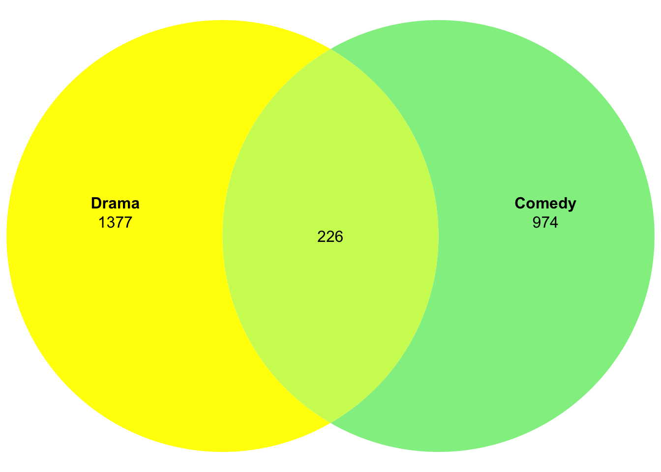
10.3 Euler diagrams
Euler diagrams are similar to Venn diagrams, with two exceptions: first, Euler diagrams try to draw every area proportional to the number of elements in the set/intersection they represent; therefore, secondly, Euler diagrams don’t include intersecting areas, if there are no elements that intersect between two sets. To demonstrate this, let’s look at another set of three genres:
movies3b <- movies[,c(5,15,17)] #keep only Children, Thriller, and Romance
rownames(movies3b) <- movies[,1]
movies3b <- movies3b[rowSums(movies3b)>0,] #remove movies that don't belong to our genres

plot(venn(movies3b),fills=c("orange","pink","purple"),edges=NA)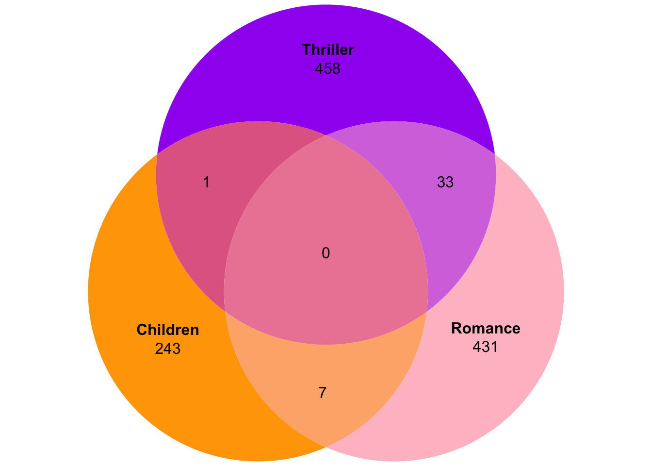
You see the 0 in the middle, meaning there are (perhaps reassuringly) no children’s movies that are also romantic thrillers. Now with the Euler diagram:
plot(euler(movies3b),fills=c("orange","pink","purple"),edges=NA,
     quantities=T)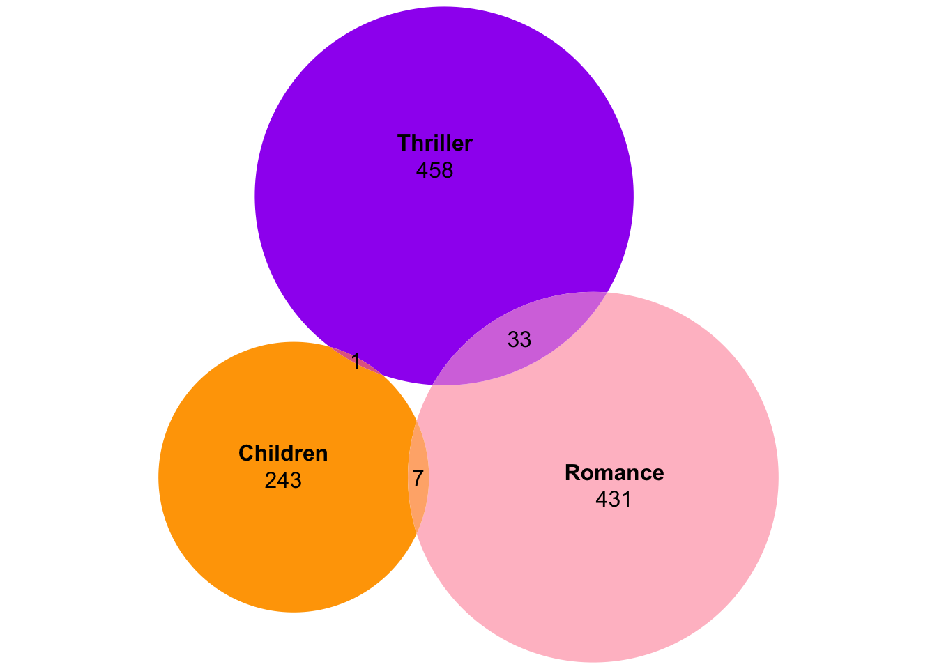
You see, there are three fields with overlaps of all pairs, and the intersection of all sets is non-existent. You also see that the circles and intersections are pretty much to scale, with the children’s circle visibly smaller than the others.
Exercise: Do the same thing for the other movies data sets we created above. Which of them can be visualized faithfully? what about the others?
10.4 UpSet plots
Euler diagrams are only guaranteed to work for two sets. After that, the
circles cannot always be drawn area-proportionally. Venn diagrams can
theoretically be plotted for many more sets, but they become really
confusing (click for an example of Venn-related
humour).
Probably, the most elegant solution to visualize the sizes of overlaps
between sets is offered by upSet plots. In R, functions are provided by
the UpSetR package. Let’s first look at the small data set from above:
upset(movies3)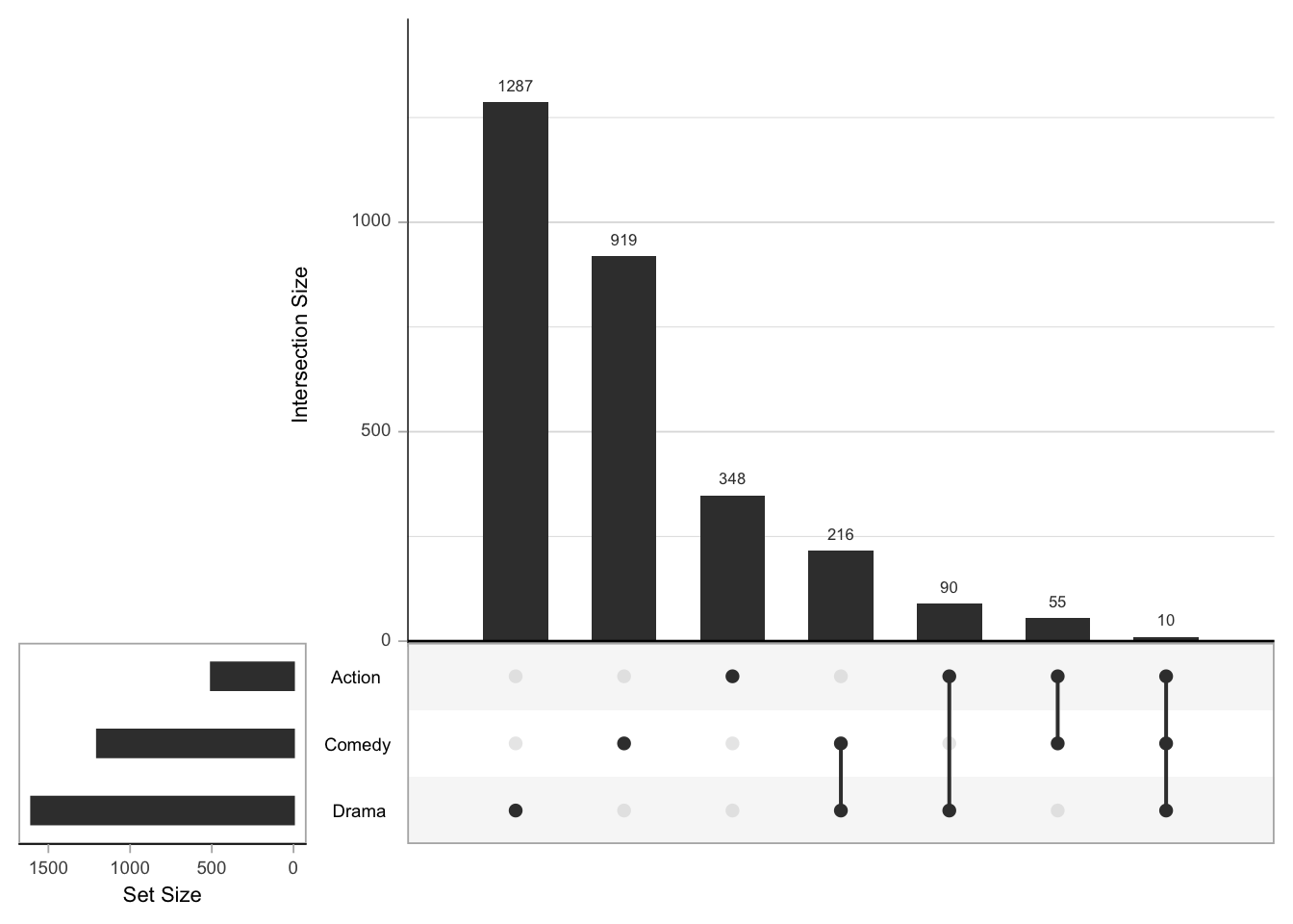
The UpSet plot is quite easy to read: at the bottom left, you have a barplot visualizing the sizes of the sets (here, the genres). To its right a black point in each set’s row means that the set belongs to a combination of sets (including the set on its own). Combinations of more than one set are emphasized by vertical lines. The barplot at the top shows the size of the combination.
Exercise: try this with our 4-genre set.
Upsets power becomes clear, when we take the whole data set (17 genres):
upset(movies, nsets = 17, nintersects = 40, mb.ratio = c(0.5, 0.5),
      order.by = "freq")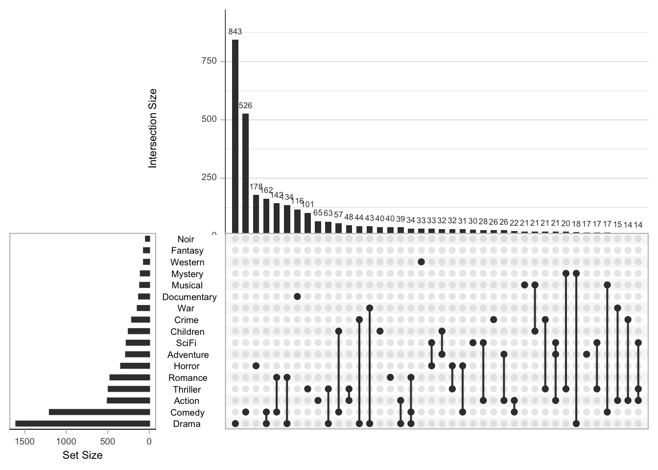
To be fair, we did not plot all of the intersects here (nintersects
argument above). But we can quickly see which genres and combinations
are most common in our database.
We can limit the number of genres like so:
upset(movies, nsets = 10, nintersects = 40, mb.ratio = c(0.5, 0.5),
      order.by = "freq")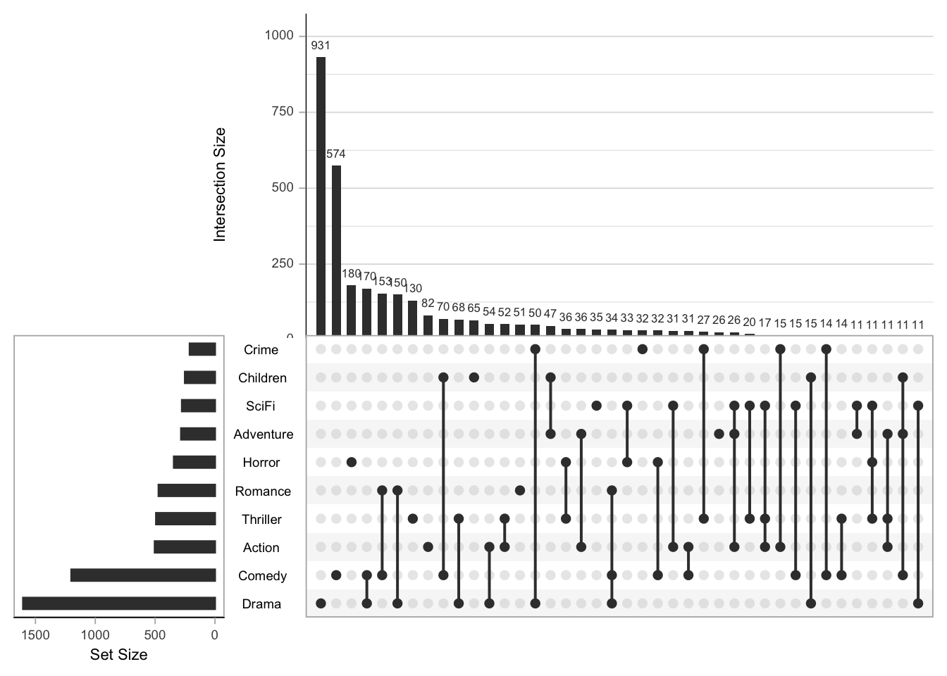
Exercise: what’s the most common 3-genre combination?
You can modify the look of the plot, by e.g. adding colours to the bars. Most of the time, these are not really informative, so we’ll not go into detail here.
You can also use the plot to summarize data in the combinations in boxplots. We could show the ratings, for example:
upset(movies, nsets = 17, nintersects = 40, mb.ratio = c(0.5, 0.5),
      order.by = "freq",
      boxplot.summary = "AvgRating")
## Warning: Continuous limits supplied to discrete scale.
## Did you mean `limits = factor(...)` or `scale_*_continuous()`?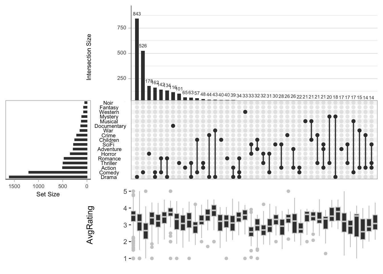
Exercise: make an upset plot with the year the movies were released shown in a boxplot.